Du fragst dich, welche Bedeutung Matrizen eigentlich haben und wie du mit ihnen rechnen kannst? Dann bist du hier genau richtig. Eine schnelle Erklärung dazu findest du in unserem Video
Matrizen einfach erklärt
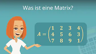
Was ist überhaupt eine Matrix? Matrizen bestehen aus Zahlen, die in m Zeilen und n Spalten angeordnet sind. Man spricht dann von einer (m x n) – Matrix bzw. einer Matrix der Dimension (m x n).
![\[A = \begin{pmatrix} a_{11} & a_{12} & \dots & a_{1n} \\ a_{21} & a_{22} & \dots & a_{2n} \\ \vdots & \vdots & \ddots & \vdots\\ a_{m1} & a_{m2} & \dots & a_{mn} \end{pmatrix}\]](https://blog.assets.studyflix.de/wp-content/ql-cache/quicklatex.com-65e4088f9530d339c59128358db29cf4_l3.png "Rendered by QuickLaTeX.com")
Dabei steht bei den Matrixeinträgen  der Index i für die Zeile und j für die Spalte der Matrix, in der sich der Eintrag befindet.
Im Prinzip ist eine (m x n) – Matrix eine vereinfachte Darstellung eines Linearen Gleichungssystems (LGS) mit m Gleichungen und n Variablen. Wenn du dann ein LGS als Matrix darstellen möchtest, verwendest du für die Matrixeinträge einfach die Koeffizienten des LGS.

Dieses LGS kannst du also mit Matrizen schreiben:
![\[\begin{pmatrix} 1 & 1 & 1 \\ 9 & 3 & 1 \\ 25 & 5 & 1 \end{pmatrix} \cdot \begin{pmatrix} x_1 \\ x_2 \\ x_3 \end{pmatrix} = \begin{pmatrix} 0 \\ 0 \\ 1 \end{pmatrix} \]](https://blog.assets.studyflix.de/wp-content/ql-cache/quicklatex.com-14c3ea21ec845917fedb2231aac41ceb_l3.png "Rendered by QuickLaTeX.com")
Dabei hat die Matrixschreibweise exakt dieselbe Bedeutung wie das LGS.
Matrix Mathe
Besondere Matrizen sind zum Beispiel:
- Quadratische Matrix: m = n
-
Diagonalmatrix: Enthält nur Nulleinträge – außer auf der Hauptdiagonalen.
Eine Diagonalmatrix ist eine quadratische Matrix, die auf der Hauptdiagonalen beliebige reelle Zahlen und ansonsten nur Nulleinträge enthält.
![\[A = \begin{pmatrix} \textcolor{blue}{1} & 0 \\ 0 & \textcolor{blue}{3} \\ \end{pmatrix} \; \; \[B = \begin{pmatrix} \textcolor{blue}{\pi} & 0 & 0 \\ 0 & \textcolor{blue}{0} & 0 \\ 0 & 0 & \textcolor{blue}{7} \\ \end{pmatrix} \]](https://blog.assets.studyflix.de/wp-content/ql-cache/quicklatex.com-ace201d0db470603ee8f70e835acc95a_l3.png "Rendered by QuickLaTeX.com")
-
Nullmatrix: Jeder Eintrag einer Nullmatrix ist Null.
Die Nullmatrix hat die Dimension (n x n) und ist das neutrale Element der Matrizenaddition.
![\[ 0_2 = \begin{pmatrix} 0 & 0 \\ 0 & 0 \end{pmatrix} \; \; 0_n = \begin{pmatrix} 0 & 0 & 0 & \dots \\ 0 & 0 & 0 & \dots \\ 0 & 0 & 0 & \dots \\ \vdots & \vdots & \vdots & \ddots \end{pmatrix} \]](https://blog.assets.studyflix.de/wp-content/ql-cache/quicklatex.com-26229394788e1dae9213829b4e0deb19_l3.png "Rendered by QuickLaTeX.com")
-
Einheitsmatrix
: Die Einträge der Hauptdiagonalen sind gleich 1, alle anderen Einträge sind gleich 0.
Die Einheitsmatrix ist eine Diagonalmatrix der Dimension
  und sie ist das neutrale Element der Matrizenmultiplikation.
![\[E_n = \begin{pmatrix} 1 & 0 & 0 &\dots \\ 0 & 1 & 0 & \dots \\ 0 & 0 & 1 & \dots\\ \vdots & \vdots & \vdots & \ddots \end{pmatrix}\]](https://blog.assets.studyflix.de/wp-content/ql-cache/quicklatex.com-369c0186d9eac2d863337d8f91c3f49a_l3.png "Rendered by QuickLaTeX.com")
-
Transponierte Matrix
: Die Transponierte
 der Matrix
  erhältst du durch Vertauschen von Zeilen und Spalten. Das heißt, die erste Spalte von ist die erste Zeile von , die zweite Spalte von ist die zweite Zeile von und so weiter.
Viele Eigenschaften wie die Spur , die Determinante , die Eigenwerte und der Rang einer Matrix bleiben unter der Transponierung unverändert (invariant).
![\[A = \begin{pmatrix} \textcolor{red}{1} & \textcolor{red}{2} & \textcolor{red}{3} \\ \textcolor{blue}{4} & \textcolor{blue}{5}& \textcolor{blue}{6} \\ \end{pmatrix} \Rightarrow \[A^T = \begin{pmatrix} \textcolor{red}{1} & \textcolor{blue}{4} \\ \textcolor{red}{2} & \textcolor{blue}{5} \\ \textcolor{red}{3} & \textcolor{blue}{6} \\ \end{pmatrix}\]](https://blog.assets.studyflix.de/wp-content/ql-cache/quicklatex.com-808db8f185937f075f4407eea079d5c5_l3.png "Rendered by QuickLaTeX.com")
-
Symmetrische Matrix: Wenn
 gilt, so ist (und damit auch ) symmetrisch.
![\[A = \begin{pmatrix} 1 & 2 & 3 \\ 2 & 7 & 4 \\ 3 & 4 & 5 \\ \end{pmatrix} = A^T\]](https://blog.assets.studyflix.de/wp-content/ql-cache/quicklatex.com-c140357da12c4ab25edc2a463b1c83a6_l3.png "Rendered by QuickLaTeX.com")
Studyflix vernetzt: Hier ein Video aus einem anderen Bereich
Nach Beantwortung speichern wir deine Antwort, um Studyflix zu verbessern. Mehr dazu erfährst du in unserer Datenschutzerklärung.
Matrizen addieren und subtrahieren
Zwei Matrizen A und B kannst du nur dann addieren oder subtrahieren, wenn beide Matrizen gleich groß sind. Als Ergebnis erhältst du erneut eine Matrix C derselben Größe. Ihre Einträge  entstehen aus den Summen bzw. Differenzen der beiden entsprechenden Einträge aus A und B.
![\[\textcolor{red}{A = \begin{pmatrix} 1 & 2 & 3 \\ 4 & 5 & 6 \\ \end{pmatrix}} \; \; \textcolor{blue}{B = \begin{pmatrix} 3 & 2 & 1 \\ 7 & 8 & 9 \\ \end{pmatrix}} \]](https://blog.assets.studyflix.de/wp-content/ql-cache/quicklatex.com-b9f9f1004cba5b318b35722ca35aa3c7_l3.png "Rendered by QuickLaTeX.com")
Dann gilt:
![\[\textcolor{red}{A} + \textcolor{blue}{B} = \begin{pmatrix} \textcolor{red}{1} + \textcolor{blue}{3} & \textcolor{red}{2} + \textcolor{blue}{2} & \textcolor{red}{3} + \textcolor{blue}{1} \\ \textcolor{red}{4} + \textcolor{blue}{7} & \textcolor{red}{5} + \textcolor{blue}{8} & \textcolor{red}{6} + \textcolor{blue}{9} \end{pmatrix}} = \begin{pmatrix} 4 & 4 & 4 \\ 11 & 13 & 15 \\ \end{pmatrix}} \]](https://blog.assets.studyflix.de/wp-content/ql-cache/quicklatex.com-1733094bccafb03e000d85846a9529be_l3.png "Rendered by QuickLaTeX.com")
und
![\[\textcolor{red}{A} - \textcolor{blue}{B} = \begin{pmatrix} \textcolor{red}{1} - \textcolor{blue}{3} & \textcolor{red}{2} - \textcolor{blue}{2} & \textcolor{red}{3} - \textcolor{blue}{1} \\ \textcolor{red}{4} - \textcolor{blue}{7} & \textcolor{red}{5} - \textcolor{blue}{8} & \textcolor{red}{6} - \textcolor{blue}{9} \end{pmatrix}} = \begin{pmatrix} -2 & 0 & 2 \\ -3 & -3 & -3 \\ \end{pmatrix}} \]](https://blog.assets.studyflix.de/wp-content/ql-cache/quicklatex.com-0c0d94a4a9c9808aebea5083f9002da7_l3.png "Rendered by QuickLaTeX.com")
Die beiden Matrizen A und C kannst du nicht addieren – wegen der unterschiedlichen Größen ist das nicht möglich.
![\[ A = \begin{pmatrix} 1 & 2 & 3 \\ 4 & 5 & 6 \\ \end{pmatrix} \; \; C = \begin{pmatrix} 3 & 2 \\ 7 & 8 \\ \end{pmatrix}} \]](https://blog.assets.studyflix.de/wp-content/ql-cache/quicklatex.com-0a0379c31e2581080bce75f46bf4bc93_l3.png "Rendered by QuickLaTeX.com")
Die Matrizenaddition ist außerdem kommutativ und assoziativ.
Matrix mal Zahl
Du kannst eine Matrix A mit jeder beliebigen Zahl r (auch Skalar genannt) multiplizieren, indem du jeden Eintrag von A einzeln mit r multiplizierst.
![\[\textcolor{blue}{r} \cdot \begin{pmatrix} 1 & 5 \\ 11 & 13 \\ 5 & 2 \end{pmatrix}} = \begin{pmatrix} \textcolor{blue}{r} & \textcolor{blue}{r} \cdot 5 \\ \textcolor{blue}{r} \cdot 11 & \textcolor{blue}{r} \cdot 13 \\ \textcolor{blue}{r} \cdot 5 & \textcolor{blue}{r} \cdot 2 \end{pmatrix}} \]](https://blog.assets.studyflix.de/wp-content/ql-cache/quicklatex.com-9223c2c561a0a5452178ed6b8c015152_l3.png "Rendered by QuickLaTeX.com")
Matrix mal Vektor
Damit du eine Matrix-Vektor-Multiplikation zwischen der Matrix A und dem Vektor v durchführen kannst, muss die Spaltenanzahl von A mit der Länge von v übereinstimmen. Du kannst eine (m x n)-Matrix also mit jedem n-dimensionalen Vektor multiplizieren. Als Ergebnis erhältst du dann einen m-dimensionalen Vektor.
![\[\textcolor{red}{A = \begin{pmatrix} 1 & 1 & 0 \\ 4 & 7 & 3 \\ \end{pmatrix}} \; \; \textcolor{blue}{v = \begin{pmatrix} 1 \\ 2 \\ 2 \end{pmatrix}} \]](https://blog.assets.studyflix.de/wp-content/ql-cache/quicklatex.com-6ded3dab1dd9298149f98df272d4429c_l3.png "Rendered by QuickLaTeX.com")
![\[ \textcolor{red}{A} \cdot \textcolor{blue}{v} = \textcolor{red}{\begin{pmatrix} 1 & 1 & 0 \\ 4 & 7 & 3 \\ \end{pmatrix}} \cdot \textcolor{blue}{ \begin{pmatrix} 1 \\ 2 \\ 2 \end{pmatrix}} = \begin{pmatrix} \textcolor{red}{1} \cdot \textcolor{blue}{1} + \textcolor{red}{1} \cdot \textcolor{blue}{2} + \textcolor{red}{0} \cdot \textcolor{blue}{2}\\ \textcolor{red}{4} \cdot \textcolor{blue}{1} + \textcolor{red}{7} \cdot \textcolor{blue}{2} + \textcolor{red}{3} \cdot \textcolor{blue}{2} \end{pmatrix}} = \begin{pmatrix} \textcolor{olive}{3} \\ \textcolor{orange}{24} \end{pmatrix}} \]](https://blog.assets.studyflix.de/wp-content/ql-cache/quicklatex.com-2b097a98fdc035298e038faede59cd66_l3.png "Rendered by QuickLaTeX.com")
Erläuterung der Rechung:
Da A so viele Spalten hat wie v Einträge, ist die Multiplikation hier möglich. Und weil A zwei Zeilen hat, erhältst du als Ergebnis einen zweidimensionalen Vektor. Um den ersten Eintrag des Ergebnisvektors zu erhalten, betrachtest du die erste Zeile von A und multipliziert den ersten Eintrag dieser Zeile mit dem ersten Eintrag von v, den zweiten Eintrag der ersten Zeile von A mit dem zweiten Eintrag von v und dasselbe mit dem dritten Eintrag der ersten Zeile von A und dem dritten Eintrag von v. Die Summe dieser drei Produkte ergibt den ersten Eintrag des Ergebnisvektors. Den zweiten Eintrag des Ergebnisvektors erhält man, wenn man für die zweite Zeile von A analog vorgeht.
Weitere Beispiele:

Matrix mal Matrix
Zwei Matrizen kannst du genau dann miteinander multiplizieren, wenn die Spaltenanzahl der ersten Matrix mit der Zeilenanzahl der zweiten Matrix übereinstimmt. Immer dann also, wenn  und
und  . Du erhältst dann als Ergebnis eine Matrix der Dimension (m x k).
![\[\textcolor{red}{A = \begin{pmatrix} 1 & 1 & 0 \\ 4 & 7 & 3 \\ \end{pmatrix}} \; \; \textcolor{blue}{B = \begin{pmatrix} 1 & 3 \\ 2 & 4 \\ 2 & 0 \end{pmatrix}} \]](https://blog.assets.studyflix.de/wp-content/ql-cache/quicklatex.com-1873aea0e43a36131d1a546a7c6a0db4_l3.png "Rendered by QuickLaTeX.com")
A hat genauso viele Spalten wie B Zeilen, also ist die Matrizenmultiplikation  durchführbar. Weil A zwei Zeilen und B zwei Spalten hat, erhältst du eine (2 x 2)-Matrix als Ergebnis.
Für den ersten Eintrag der ersten Spalte der Ergebnismatrix betrachtest du die erste Zeile von A und die erste Spalte von B. Dann gehst du vor wie bei der Matrix-Vektor-Multiplikation – du rechnest also „Zeile mal Spalte“.
![\[\textcolor{red}{A} \cdot \textcolor{blue}{B} = \textcolor{red}{\begin{pmatrix} 1 & 1 & 0 \\ 4 & 7 & 3 \\ \end{pmatrix}} \cdot \textcolor{blue}{ \begin{pmatrix} 1 & 3 \\ 2 & 4 \\ 2 & 0 \end{pmatrix}} = \begin{pmatrix} \textcolor{red}{1} \cdot \textcolor{blue}{1} + \textcolor{red}{1} \cdot \textcolor{blue}{2} + \textcolor{red}{0} \cdot \textcolor{blue}{2} & *\\ * & * \end{pmatrix}} = \begin{pmatrix} 3 & *\\ * & * \end{pmatrix}} \]](https://blog.assets.studyflix.de/wp-content/ql-cache/quicklatex.com-898402e24b5e611923de3a4b5b1ef9fb_l3.png "Rendered by QuickLaTeX.com")
Den ersten Eintrag der zweiten Spalte erhältst du, wenn du die erste Zeile von A und die zweite Spalte von B betrachtest und die gleichen Rechenschritte durchführst.
![\[\textcolor{red}{A} \cdot \textcolor{blue}{B} = \textcolor{red}{\begin{pmatrix} 1 & 1 & 0 \\ 4 & 7 & 3 \\ \end{pmatrix}} \cdot \textcolor{blue}{ \begin{pmatrix} 1 & 3 \\ 2 & 4 \\ 2 & 0 \end{pmatrix}} = \begin{pmatrix} 3 & \textcolor{red}{1} \cdot \textcolor{blue}{3} + \textcolor{red}{1} \cdot \textcolor{blue}{4} + \textcolor{red}{0} \cdot \textcolor{blue}{0}\\ * & * \end{pmatrix}} = \begin{pmatrix} 3 & 7\\ * & * \end{pmatrix}} \]](https://blog.assets.studyflix.de/wp-content/ql-cache/quicklatex.com-124009d6807cbfdbf83e534cb68205d2_l3.png "Rendered by QuickLaTeX.com")
Um den zweiten Eintrag der ersten Spalte der Ergebnismatrix zu berechnen, multipliziere die zweite Zeile von A mit der ersten Spalte von B.
![\[\textcolor{red}{A} \cdot \textcolor{blue}{B} = \textcolor{red}{\begin{pmatrix} 1 & 1 & 0 \\ 4 & 7 & 3 \\ \end{pmatrix}} \cdot \textcolor{blue}{ \begin{pmatrix} 1 & 3 \\ 2 & 4 \\ 2 & 0 \end{pmatrix}} = \begin{pmatrix} 3 & 7\\ \textcolor{red}{4} \cdot \textcolor{blue}{1} + \textcolor{red}{7} \cdot \textcolor{blue}{2} + \textcolor{red}{3} \cdot \textcolor{blue}{2} & * \end{pmatrix}} = \begin{pmatrix} 3 & 7\\ 24 & * \end{pmatrix}} \]](https://blog.assets.studyflix.de/wp-content/ql-cache/quicklatex.com-3232bf05deeac7a34e534207fa6527a4_l3.png "Rendered by QuickLaTeX.com")
Und für den zweiten Eintrag der zweiten Zeile der Ergebnismatrix multipliziere die zweite Spalte von A mit der zweiten Spalte von B.
![\[\textcolor{red}{A} \cdot \textcolor{blue}{B} = \textcolor{red}{\begin{pmatrix} 1 & 1 & 0 \\ 4 & 7 & 3 \\ \end{pmatrix}} \cdot \textcolor{blue}{ \begin{pmatrix} 1 & 3 \\ 2 & 4 \\ 2 & 0 \end{pmatrix}} = \begin{pmatrix} 3 & 7\\ 24 & \textcolor{red}{4} \cdot \textcolor{blue}{3} + \textcolor{red}{7} \cdot \textcolor{blue}{4} + \textcolor{red}{3} \cdot \textcolor{blue}{0} \end{pmatrix}} = \begin{pmatrix} 3 & 7\\ 24 & 40 \end{pmatrix}} \]](https://blog.assets.studyflix.de/wp-content/ql-cache/quicklatex.com-cc8f8affce6f5147992c079f9b5b2626_l3.png "Rendered by QuickLaTeX.com")
Das ist das Ergebnis der Matrizenmultiplikation .
Du solltest dabei aber immer bedenken, dass die Matrixmultiplikation im Allgemeinen nicht kommutativ ist.
Beispielrechnungen:

Die Division, wie wir sie aus den reellen Zahlen kennen, ist mit Matrizen übrigens nicht möglich. Statt durch eine Matrix A zu dividieren, musst du mit ihrer Inversen Matrix
 multiplizieren (falls es diese gibt).
Matrizen — häufigste Fragen
(ausklappen)
Matrizen — häufigste Fragen
(ausklappen)-
Wie multipliziert man Matrizen?Matrizen multiplizierst du, indem du zu jedem Ergebnis-Eintrag eine Zeile der ersten Matrix mit einer Spalte der zweiten Matrix verrechnest (Produkte bilden und addieren). Das geht nur, wenn die Spaltenzahl der ersten zur Zeilenzahl der zweiten passt. Beispiel:
![\begin{pmatrix}1 & 0 & 2\\-1 & 3 & 1\end{pmatrix}\!\cdot\!\begin{pmatrix}2 & 1\\0 & -1\\1 & 4\end{pmatrix} = \begin{pmatrix} 1\cdot2 + 0\cdot0 + 2\cdot1 & 1\cdot1 + 0\cdot(-1) + 2\cdot4\\[4pt] -1\cdot2 + 3\cdot0 + 1\cdot1 & -1\cdot1 + 3\cdot(-1) + 1\cdot4 \end{pmatrix} = \begin{pmatrix}4 & 9\\-1 & 0\end{pmatrix}.</td> </tr> <tr> <td style="width: 50%;"><strong>Wie multipliziert man zwei 2×2-Matrizen?</strong></td> <td style="width: 50%;">Zwei](https://blog.studyflix.de/wp-content/ql-cache/quicklatex.com-007a08e9850d759746caa810502786c6_l3.png "Rendered by QuickLaTeX.com") 2\times2
2\times2 (1,1)
(1,1) (1,2)(2,1)(2,2)
 \begin{pmatrix}1 & 2\\3 & 4\end{pmatrix}\!\cdot\!\begin{pmatrix}0 & 5\\6 & 7\end{pmatrix} = \begin{pmatrix}
1\cdot0 + 2\cdot6 & 1\cdot5 + 2\cdot7\\[4pt]
3\cdot0 + 4\cdot6 & 3\cdot5 + 4\cdot7
\end{pmatrix} = \begin{pmatrix}12 & 19\\24 & 43\end{pmatrix}.
\begin{pmatrix}1 & 2\\3 & 4\end{pmatrix}\!\cdot\!\begin{pmatrix}0 & 5\\6 & 7\end{pmatrix} = \begin{pmatrix}
1\cdot0 + 2\cdot6 & 1\cdot5 + 2\cdot7\\[4pt]
3\cdot0 + 4\cdot6 & 3\cdot5 + 4\cdot7
\end{pmatrix} = \begin{pmatrix}12 & 19\\24 & 43\end{pmatrix}.
-
Kann man 3 Matrizen multiplizieren?Drei Matrizen kannst du multiplizieren, wenn die Dimensionen in der gegebenen Reihenfolge zusammenpassen, und du rechnest dann in zwei Schritten. Du darfst dabei klammern, also erst
 oder
oder  , aber du darfst die Reihenfolge nicht einfach vertauschen. Beispiel:
  ,
,  ,
,  ergibt in beiden Klammerungen einen
  -Vektor.
Determinante
Jetzt kennst du dich mit der Bedeutung und der Berechnung von Matrizen aus. Für deine nächste Prüfung könnte es aber auch sehr hilfreich sein, dir unseren Artikel über Determinanten von Matrizen anzusehen.
